The last years have seen a rapid rise in the number of web sites that support a "dark mode". Some pages offer an explicit light/dark switch. But typically the selection is based on the browsers "prefers-color-scheme" CSS selector. It is surprisingly difficult to change this browser default without switching the whole operating system.

Follow the instructions below to switch to dark mode.

Chrome

For Chrome, the instructions depend on the system it is running on.

On Android

• In Chrome, open the top-right "..." menu and go to "Settings"
• Open "Themes"
• Select "Dark"

On iOS

There is no direct way to enable dark mode only for Chrome on iOS. You have to change the whole device to iOS via "Settings" → "Display & Brightness".

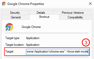
On Windows

Chrome switches into dark mode when it is started with the --force-dark-mode command line flag.

• Close all Chrome instances
• Shift-Right click the Chrome shortcut in the taskbar or on the desktop
• Select "Properties"
  
• In the "Shortcut" tab, append --force-dark-mode to the "Target" field
• Close the dialog with "OK"
  
• Restart Chrome with that shortcut

Safari

Safari doesn't have a separate setting for dark mode. It always follows the operating system setting.

Changing the system setting on iOS

• Open Settings
• Open "Display & Brightness"
• Select "Dark"

Changing the system setting on MacOS

• Open the system settings in the Apple menu
• Open the "General" dialog
• Select the "Dark" appearance

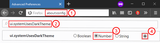
Firefox

Firefox has hidden configuration option that enables dark mode:

• Type about:config into the address bar and press Enter
• Type ui.systemUsesDarkTheme into the search bar
• The search will not find anything, but allow you to add a new preference with that name

• Set the property type to "Number" and click the "+" button to create:
  

• Enter the value "1" to enable dark mode and click the check mark to save:
  

Administrating an LDAP server may be hard — using it doesn't have to be.

LDAP servers commonly provide auth services to web servers, mail servers, web apps, and so on. To do this, the LDAP database stores user and group membership information. The combination of these two datasets allows both authentication (is the user who they claim to be?) and authorization (is the user in a group that has permission to perform a specific action?). Thus, LDAP enables central management of user, group, and permission information for any number of services.

Concepts

So what does an LDAP database consist of?

• An LDAP database contains a hierarchical data structure, similar to a directory tree.
• Each tree node is called an entity.
  • LDAP doesn't distinguish between files and directories. Entities often contain both child entities — like a directory — as well as attributes, which are similar to a file's content.
• Each entity has a distinguished name (DN), which is the entity's absolute pathname in LDAP tree. The elements of the pathname are called relative distinguished names (RDNs).
  These concepts are pretty similar to filesystem directory trees. The key differences are:
  • Directory separators: LDAP uses , instead of /
  • RDN format: RDNs are typically key-value-pairs, instead of simple strings: uid=ca instead of Desktop. Commonly used keys are dc, o, ou, uid.
  • Parent nodes are on the right: so it's dc=child,dc=parent instead of /parent/child
    Consequently, DNs usually look like this: uid=ca,ou=people,dc=caichinger,dc=com
• Entities have attributes, which store the entity's data, similar to a file's contents. Each attribute has a type that describes the attribute's data structure, as well as one or more values containing the attribute's information. Additionally, each attribute can have options — a rarely used feature for distinguishing different versions (e.g. English, German) of the same attribute.
• Entities also have associated object classes, which are conceptually similar to attribute types. But whereas types describe attributes, object classes describe which attributes must be found within the entity.
• Both attribute types and entity object classes are metadata: they describe the database's schema. Each of these metadata objects has an OID. Aside from the schema definition, OIDs are also used for other database-specific metadata, such as identifying extended requests and responses. OIDs are denoted as dot-separated numbers, e.g. 1.2.840.1234567890, but often have human-readable names assigned as well.

What actions can be performed over the LDAP protocol?

• Binding: authenticating to the LDAP server — essentially "logging in". Since most servers don't allow un-authenticated querying, this is required before performing any other actions. Many servers also support re-authentication as a different user over existing connections: this is known as re-binding.
• Searching: querying the existing LDAP directory tree, and listing its information.
• Add, modify, and delete: altering the LDAP directory tree.
• Many others, often including custom commands.

Querying

Querying an LDAP server is straight-forward with the ldapsearch tool:

ldapsearch
  -h ldap.caichinger.com                       # LDAP server name
  -D "uid=ca,ou=people,dc=caichinger,dc=com"   # Authenticate as uid=caichinger
  -W                                           # Ask for password for uid=caichinger
  -b "ou=people,dc=caichinger,dc=com"          # Base search path
  (uid=caichinger)                             # Search expression

The -D and -W switches tell ldapsearch as which user to authenticate as. The -b switch defines the "base directory" where the search should start. The search expression is then applied to all entities under this directory tree.

The server response will then contain all matching users, as well as their associated attributes.

If you have any questions after this whirlwind-tour of LDAP, please leave a comment!

Sometimes, we need to convert Unix timestamps (seconds since January 1st, 1970) to human-readable dates. For example, we might transform 1539561600 to 2018-10-15 00:00 UTC.

There are multiple online services that do this, I like unixtimestamp.com.

Every now and then we need to batch-convert timestamps. The date command shipped on Linux distributions does this nicely:

date "+%c" --date=@1539561600

I recently ran into a similar problem when logfiles contained Unix timestamps instead of human-readable dates. Using date seemed a bit clumsy here. Fortunately, Superuser.com had a nice solution involving Vim. The following sequence converts the timestamp under the cursor and records a macro q to facilitate future conversions:

qq                             " start recording
"mciw                          " put time in register m and replace it…
<C-r>=strftime("%c", @m)<CR>   " …with localized datetime
<Esc>                          " exit insert mode
q                              " stop recording

Quick and convenient — and easily incorporated into a macro to convert timestamps across the entire file.

This is the final post in a four-part series exploring the Kelly criterion:

• The Kelly Criterion: Introduction
• The Kelly Criterion: Multiple Investment Opportunities
• The Kelly Criterion: Where does the logarithm come from?
• The Kelly Criterion: Comparison with Expected Values (this post)

In a previous post, we looked at the Kelly formula, which maximizes earnings in a series of gambles where winnings are constantly re-invested. Is this equivalent to maximizing the expected return in each game? It turns out that the answer is "no". In this post we'll look into the reasons for this and discover the pitfalls of expected values.

We will look at the same game as in the previous post:

with the variables:

• $V_0, V_1$: the available money before and after the first round
• $l$: fraction of available money to bet in each round (the variable to optimize)
• $r_W, r_L$: return on win and loss, 0.4 and -1 in our example (i.e. 40% of wager awarded on win, otherwise 100% of wager lost)
• $W$: Random variable describing our chances to win; valued $1$ with $p=0.8$, $0$ with $p=0.2$

The Kelly formula obtained from maximizing $\log V_1/V_0$ tells us to invest 30% of our capital in such a gamble. Let's see what the result is if we maximize the expected value $E[V_1/V_0]$ instead.

This is trivial by hand, but we'll use SymPy, because we can:

import sympy as sp
import sympy.stats as ss
sp.init_printing()

l = sp.symbols('l')             # Define the symbol/variable l
W = ss.Bernoulli('W', 0.8)      # Random variable, 1 with p=0.8, else 0
def f1(W):                      # Define f1 = V_1/V_0
    return (1 + 0.4*l)**W * (1 - l)**(1-W)
ss.E(f1(W))                     # Calculate the expected value

Evaluating this gives:

Uh-hum... so the expected return has no maximum, but grows linearly with increasing $l$. Essentially, this approach advises that you should bet all your money, and more if you can borrow it for negligible interest rates.

Could the problem be that we only look at a single round? Let's examine the expected return after playing 10 rounds:

# Note: We can not do f10 = f1(W)**10, since we need independent samples
W_list = [ss.Bernoulli('W_%d' % i, 0.8) for i in range(10)]
f10 = sp.prod([f1(Wi) for Wi in W_list])
sp.expand(ss.E(f10))

All the coefficients of the polynomial are positive, there are no maxima for $l >= 0$. What's going on?

Time to dig deeper. Let's say we bet all of our money each round. If we lose just once, all of our money is gone. After 10 rounds playing this strategy, the probability of total loss is:

So 89% of the time we would lose all our money. However, the expected return after 10 rounds at $l=1$ is:

So on average we'd have $3.10 after 10 rounds for every Dollar initially bet, but 90% of the time we'd lose everything. Strange.

The big reveal

Things become clearer when we look at in more detail at the calculation of $E[V_{10}/V_0]$:

The expected value is the sum of probability-weighted outcomes($1.4$ and $0$ are the per-round outcomes for win and loss). Since a single loss results in loss of all money, the only non-zero term in the sum is the starred one, that occurs with about 11% probability, at a value gain of $1.4^{10} = 28$. This high gain is enough to drag the expected return up to 3.1. When more then 10 rounds are played, these numbers become more extreme: the winning probability plummets, but the winning payoff skyrockets, dragging the expected return further upwards.

This is a bit reminiscent of the St. Petersburg paradox, in that arbitrarily small probabilities can drag the expected return to completely different (read "unrealistic") values.

Different kinds of playing

The Kelly approach builds on the assumption that you play with all your available wealth as base capital, and tells you what fraction of that amount to invest. It requires reinvestment of your winnings. Obviously, investing everything in one game ($l=1$) is insane, since a single loss would brankrupt you. However, following Kelly's strategy is the fastest way to grow total wealth.

The expected-value approach of "invest everything you have" is applicable in a different kind of situation. Let's say you can play only one game per day, have a fixed gambling budget each day, and thus are barred from reinvesting your wins. If you invest your full daily gambling budet, you may win or lose, but over the long run you will average a daily return of $1.4 \cdot 0.8 = 1.12$ for every dollar invested. The more you can invest per day, the higher your wins, thus the pressure towards large $l$ values.

In a way, Kelly optimizes for the highest probability of large returns when re-investing winnings, while the expected value strategy optimizes for large returns, even if the probability is very low.

A dubious game

Should you play a game where the winning probability $p$ is $10^{-6}$, but the winning return $r_W$ is $2\cdot 10^6$? Mathematically it seems like a solid bet with a 100% return on investment in the long run. The question is whether you can reach "the long run". Can you afford to play the game a million times? If not, you'll most likely lose money. If you can afford to play a few million times, it becomes a nice investment indeed.

Kelly would tell you to invest only a very small fraction of your total wealth into such a game. The expected-value formalism advises to invest as much as possible, which for most people is bad advice even when playing with a fixed daily budget and no reinvestment (i.e. the expected-value play style).

This is an interesting example for two reasons:

• It demonstrates one of the ways how "rich become richer" - the game has high returns, but also a significant barrier to entry.
• It demonstrates a downside of both the Kelly- and the expected-value approach. The two strategies are optimal in their use cases in the limit of infinitely many games, however for finitely many games they may give bad advice, especially regarding to very low-probability winning scenarios.

Conclusion

So, a brief discussion of the relationship between the Kelly strategy and the expected return. For me, it was striking how two seemingly similar approaches ("maximize the moneys") lead to so different results and how unintuitively the expectation value can be in the face of outliers.

If you're interested in interactive plots that really helped me understand this material, you can find them in this Jupyter Notebook.

The Kelly criterion

Over the course of this blog post series, we looked at the classical Kelly criterion in the first post, and how it can be extended to situations such as stock buying, with multiple parallel investment opportunities, in the second post. Next, we investigated the origin of the logarithm in the Kelly formula in the third post, before finishing up with the current discussion about expected values.

Surely, there's more to say about the Kelly criterion. If you want to leave your thoughts, please do so in the comments below!

This is the third post in a four-part series exploring the Kelly criterion:

• The Kelly Criterion: Introduction
• The Kelly Criterion: Multiple Investment Opportunities
• The Kelly Criterion: Where does the logarithm come from? (this post)
• The Kelly Criterion: Comparison with Expected Values

The neat thing about the derivations in the last two posts is that they give a motivation for "optimizing the logarithm of wealth". The logarithm is not put in by decree, but is a mathematical technicality that arises from the repeated betting process! Kelly mentions this in his original paper:

At every bet he maximizes the expected value of the logarithm of his capital. The reason has nothing to do with the value function which he attached to his money, but merely with the fact that it is the logarithm which is additive in repeated bets and to which the law of large numbers applies.

This argument is very general. Let's say we model the wealth $V_n$ after $n$ rounds of betting based on the initial wealth $V_0$ in terms of a function $f(R, l) = V_{n+1} / V_n$ as

where $R$ is a random variable describing the possible outcomes of the game, and $l$ is the fraction of available money to invest in each round. Then we can derive the following formula for the best $l$ value:

where $r_j$ are the possible investment outcomes and $p_j$ are the associated probabilities. The crucial change from random variable $R$ to outcomes and probabilities $r_j$ and $p_j$ is justified by the law of large numbers. Based on the exponential nature of the formula, switching to a logarithmic view feels very natural.

Consequently, neither the details of the game — represented by the random variable $R$ — nor the exact form of the per-round return $f$ matter. Any iterative scheme with reinvestment of profits should be representable in the form of equation (1), leading to the logarithm in solution (2). Beyond the origin of the logarithm, this analysis also shows the universality of the Kelly derivation.

Unfortunately, this argument is mostly skipped in online discussions. Often the logarithm is not justified at all, or it is treated as "genius from the 1950s says: use $\log$". Sometimes the result is also linked to utility theory, which posits that having twice the money is not twice as useful. While utility theory may be true, reasonable people can disagree on their utility function — exactly how useful more or less money is to them. However, Kelly's result is not grounded in utility, and the $\log$ does not represent logarithmic utility of money. Consequently, even people who disagree on their utility function should agree that the Kelly criterion is the fastest way to gain wealth.

I hope this post shed some light on the reasoning behind the Kelly decision scheme. If you're interested in interactive plots that really helped me understand this material, you can find them in this Jupyter Notebook.

In the next post, we'll take a closer look at the relation of the Kelly criterion to expected values.